
In this project, we developed a new method for determining the refractive index of dynamic droplets in a spray using a machine learning approach, in which the four light scattering signals of individual droplets were analyzed.
The spray was produced using a flat fan nozzle, and to vary the refractive index, a water-glycerin mixture with different mixing ratios was used. First, a machine learning model was developed to analyze the four light scattering signals. In addition, we investigated whether the number of signals could be reduced while maintaining prediction accuracy.
The measurement of individual static droplets, for example when a droplet is levitated acoustically or electromagnetically, can be done by analyzing rainbow scattering. However, determining the refractive index of individual dynamic droplets within a flow remains a major challenge, as there are currently no commercial instruments capable of performing this measurement.
This project proposes the use of machine learning to extend this method by analyzing signal shape, enabling TSTOF devices to characterize the refractive index of individual dynamic droplets in real time.
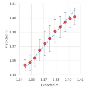
Results Using a machine learning approach and experimental data, a model was created. The trained model was applied to a test dataset, and the final result is shown in Figure 1. The predicted values are presented as a statistical ensemble with a mean and standard deviation.
When comparing a large number of individual droplets made of different materials, the predicted mean values of the refractive index can be used to distinguish materials with a refractive index difference as small as 0.005. For example, water droplets with m(λ=405 nm)=1.34 and ethanol droplets with m(λ=405 nm)=1.37 can be clearly separated and classified using the method presented in this study.
ML Approach In this study, we used four steps to build the machine learning model:
- Data preparation
- Clustering with k-means
- Training with CNN
- Validation and testing
Data Preparation From a single dataset recorded by a digital oscilloscope, individual droplet light scattering signals were segmented to create a dataset in which each droplet signal was paired with a refractive index label. The segmentation process was based on a threshold set for a single channel, and parameters such as trigger threshold, signal window length, and pre-trigger were defined. Offsets were adjusted to integrate all four signals into the window, as the position of the signal was not relevant for this task. A 280 kHz low-pass Fourier filter was applied to reduce noise before loading the dataset.
Clustering with k-Means Non-informative signals caused by oscilloscope errors may occur and should not be used for training or predictions. These were removed using the k-means clustering algorithm.
In this approach, signals were represented as vectors, with centroids randomly placed in the signal space using Euclidean distance. Clusters were formed by assigning signals to the nearest centroid. The centroids were iteratively updated until stable clusters emerged.
The four light scattering signals of a single droplet were flattened into one-dimensional vectors with 22,000 samples. The optimal number of centroids was determined using the elbow method. Then, the k-means clustering algorithm was applied, and signals that exceeded a defined distance to their nearest centroid were removed.
To further improve model accuracy, clusters with a high proportion of poor predictions were identified and excluded, and the model was retrained. This approach was effective for large datasets with many poor predictions but did not improve performance for already well-performing datasets.
Training with CNN Since the refractive index of the liquid can be derived from the shape of the scattering signals, it was logical to use a neural network architecture based on convolutional layers. Convolutional Neural Networks (CNNs) are commonly used in one-dimensional signal analysis because they work well with spatial features and support efficient pattern recognition.
Four preprocessed light scattering signals of individual droplets, each with 5,500 samples, were fed into the neural network. The architecture used for this task is shown in Figure 2 and consists of 16 blocks, alternating between 8 convolutional layers and 8 max-pooling layers. Each convolutional layer had a kernel size of 7 and included batch normalization and ReLU activation. The first max-pooling layer had a kernel size of 4, while the remaining ones used a size of 2.
After the first layer, a max-pooling layer reduced the signal size by a factor of 8. After the second, third, and fourth layers, additional max-pooling layers reduced the size by a factor of 4 each.
The resulting feature maps were then flattened and passed to a fully connected neural network consisting of two linear layers with a dropout layer in between. The output of the network was a predicted value for the refractive index.
To improve convergence during training and prevent overfitting, techniques such as weight decay and uniform Xavier initialization were also used. The loss function was defined as the mean squared error, with additional weighting applied to emphasize predictions where the model typically performed poorly.
Validation and Testing Training and testing were performed on different datasets with varying trigger thresholds for signal segmentation, resulting in different minimum signal amplitudes. This was done to determine the optimal trigger threshold, which was varied from 11.5% to 21.5% in 2% increments. Dataset sizes ranged from approximately 17,000 to 32,000 signals.
The influence of the number of channels containing information for training and prediction accuracy was also examined. Training was conducted with four, three, two, and one channel using the same architecture. In total, 15 combinations of different channels and corresponding model weights were tested. The results are shown as graphs with average loss values for each model. The average loss value was determined by testing each model on the same test dataset of 3,200 signals (see Figure 2). Two loss metrics are reported: mean squared error (MSE) and the average loss used during training.