In this project, we developed a new instrument combined with a machine learning approach to realize a more cost-effective and compact measurement device for dynamic particle characterization in sprays. This is based on the Time-Shift Time-of-Flight (TSTOF) technique.

Approach

Based on the mathematical description of light scattering signals in a TSTOF device, it is known that particle size and velocity can be calculated from a single light scattering signal. Therefore, it is theoretically unnecessary to capture all four light scattering signals that are typically required in the classical computation approach of the TSTOF technique; capturing just one signal is sufficient.

The main goal of this work was to develop a machine learning approach to extract this information from a single light scattering signal. A previous study proposed using a Gaussian fit for a light scattering signal. This allowed the extraction of information about particle size and velocity from just one signal.

By fitting the light scattering signal, we were able to determine the exact temporal positions and widths of the signal, enabling us to calculate the particle size and velocity. Since the computation time for fitting functions can be unpredictable and lengthy, the use of a pre-trained machine learning model is proposed. In addition, the long calculation time is not practical for real-time analysis of particles at high throughputs—such as 150,000 particles per second—that typical commercial devices can handle.

Implementation

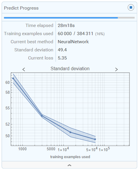
The machine learning model in this project was trained using neural network regressions. Measurement data from a full dataset of 384,311 individual light scattering signals from a single channel was used for training. A separate measurement dataset, not included in the training data, was used for testing the model.

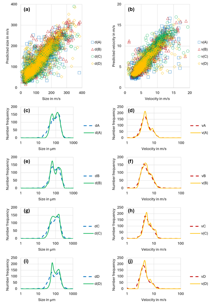
To validate the trained machine learning model, we used the light scattering signals of 12,344 particles. To increase the diversity of the test data, an additional 1,000 randomly selected light scattering signals were included.

The input and predicted values are shown in Figure 1 (a) for particle size and in Figure 1 (b) for particle velocity. Ideally, these values would lie on a straight line in a perfect prediction. The distributions are shown in Figure 2 (a–j), highlighting the performance of the model.